Estimation

This section describes how to estimate the electrical field in focal plane in Asterix. Several estimation mode are possible in Asterix. Additional details can be found directly in the code documentation.

It contains 2 functions at least:

an initialization Estimator.__init__() The initialization will require previous initialization of the testbed (see previous section) and the [Estimationconfig] part of the parameter file. It set up everything you need for the estimation (e.g. the PW matrix).
an estimation function itself with parameters:
- the entrance EF
- DM voltages

It returns the estimation as a 2D complex array. The size in pixel of the output is set by the Estim_bin_factor parameter and is dimScience / Estim_bin_factor.

from Asterix.wfsc import Estimator
# testbed is previously defined

Estimationconfig = config["Estimationconfig"]

myestim = Estimator(Estimationconfig, testbed)
resultatestimation = myestim.estimate(testbed,
                                      voltage_vector=init_voltage,
                                      entrance_EF=input_wavefront)

estimate function has been set up with a mode where each optical plane is saved to .fits file for debugging purposes. To use this option, set up the keyword dir_save_all_planes to an existing path directory.

Perfect Estimation

This is a perfect estimation in focal plane of the electrical field in focal plane. You can use this estimation by setting the parameter estimation='Perfect' before initialization. However, this estimation can be also done wihtout initialization or if another estimation have been initialized:

from Asterix.wfsc import Estimator

# testbed is previously defined
Estimationconfig = config["Estimationconfig"]

# we initialize in perfect mode
Estimationconfig.update({'estimation': "Perfect"})
myestim = Estimator(Estimationconfig, testbed)
resultatestimation = myestim.estimate(testbed,
                                      voltage_vector=init_voltage,
                                      entrance_EF=input_wavefront)
# this is a perfect FP estimation

# we re- initialize in pair-wise mode
Estimationconfig.update({'estimation': "pw"})
myestim = Estimator(Estimationconfig, testbed)

resultatestimation = myestim.estimate(testbed,
                                      voltage_vector=init_voltage,
                                      entrance_EF=input_wavefront)
# this is a pair-wise FP estimation

resultatestimation = myestim.estimate(testbed,
                                      voltage_vector=init_voltage,
                                      entrance_EF=input_wavefront,
                                      perfect_estimation=True)
# this is also a perfect FP estimation, without
# re-initializing the estimator

The perfect estimation is exactly equivalent to propagate the light throught the testbed and then resized by the Estim_bin_factor:

from Asterix.utils import resizing
# testbed is previously defined

resultatestimation = resizing(testbed.todetector(voltage_vector=init_voltage,
                              entrance_EF=input_wavefront),myestim.dimEstim)

All estimators are done this way (first obtains images in the focal plane at the Science_sampling and then resizing) to ensure that the behavior is equivalent to waht would be done on a real testbed

Pair Wise Estimation

The Pair wise estimation version we used is defined in Potier et al. (2020) The probe used are actuators, which can be chosen using posprobes parameter. If you choose 2 random actuators, it can be useful to check the .fits file starting in EigenValPW in Interaction_Matrices directory. This is the map of the inverse singular values for each pixels and it shows if all of the part of the DH are covered by the estimation (see Fig. 4 in Potier et al. 2020).

Polychromatic Estimation

We recall that polychromatic images are parametrized in [modelconfig]. We use nb_wav simulation wavelengths in Delta_wav, centered on wavelength_0 and then use the Riemann sum to approximate the polychromatic image. If mandatory_wls is an empty list (mandatory_wls = ,), these simulation wavelengths are evenly spaced. Polychromatic estimation and correction are linked so they are both driven by the parameter the [Estimationconfig] section, polychromatic:

'singlewl': only one wavelength is used for estimation / correction. Probes and PW / EFC matrices are measured at this wavelength. This parameter allows you to test the results of a monochromatic correction, applied to polychromatic light.
'broadband_pwprobes': This is mostly like the previous case, but probes images used for PW are broadband (of bandwidth Delta_wav). Matrices are at central wavelength. This is what is currently done in Potier et al. (2022) on SPHERE on sky for example. This mode is only relevant for PW estimation and will raise an error if use with perfect estimation.
'multiwl': several images at different wls are used for estimation and there are several matrices of estimation. This parameter is only for the estimation / correction. The bandwidth of the images are still parametrized in [modelconfig](nb_wav, Delta_wav)

We have 2 ways of defining the estimation / correction wavelengths. If polychromatic = 'broadband_pwprobes', the central wavelength and bandwidth are always used. For other case, you can use 2 different methods :

Method 1 (preferable for beginners): automatic selection. If no estimation_wls are hand-picked estimation_wls = , the estimation / correction wavelengths are automatically estimated.

If polychromatic = 'singlewl' the central wavelength is used. If polychromatic = 'multiwl' the wavelengths are automatically selected to be equally distributed in the bandwidth [modelconfig](Delta_wav) parameter. We use nb_wav_estim estimation / correction wavelengths evenly spaced in Delta_wav, centered on wavelength_0, the same way that the nb_wav simulation wavelengths are defined. These wavelength must be sub parts of the simulated wavelengths because a lot of wavelength specific tools are defined during OpticalSystem initialization. For this reason nb_wav_estim must be an odd integer, divisor of nb_wav. The next figure shows nb_wav = 9 for the wavelength of simulation in blue and nb_wav_estim = 3 for the wavelengths of estimation / correction in red.

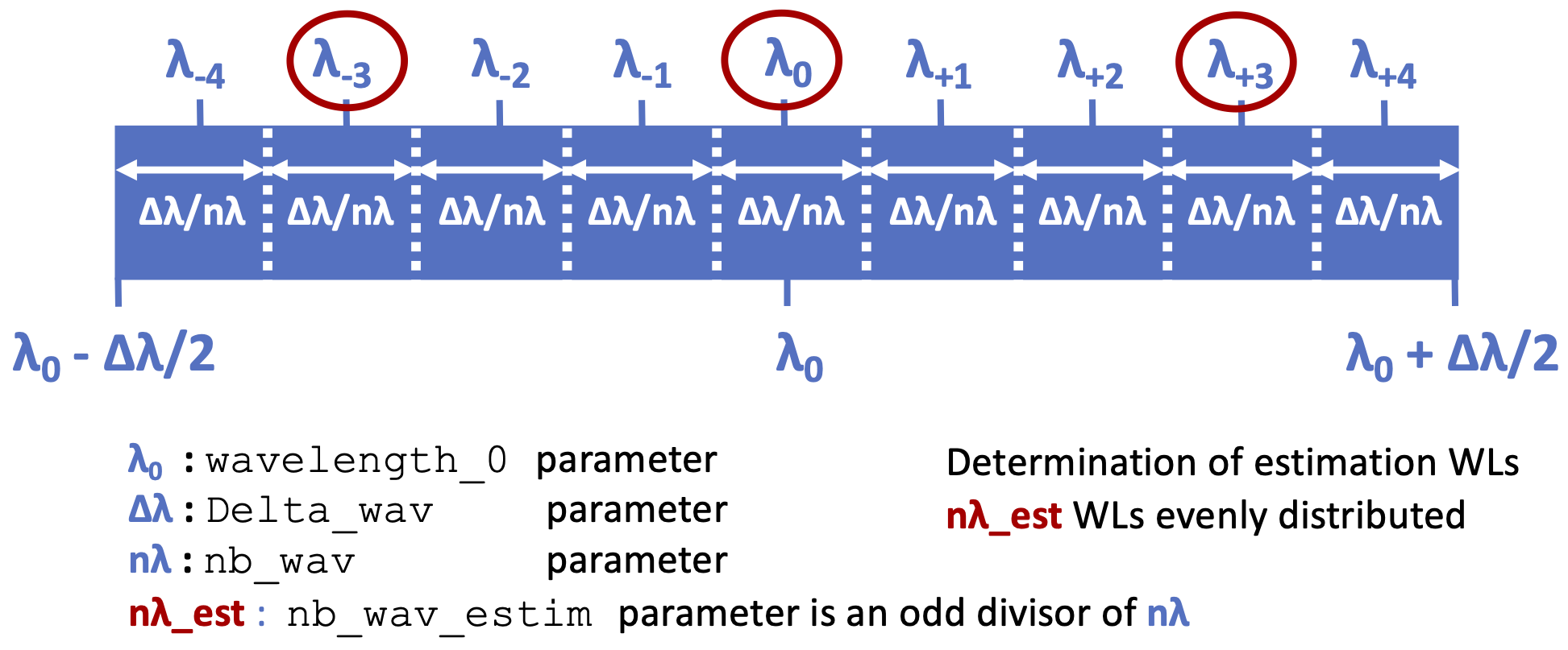
_images/wl_estim.png — Determination of estimation wavelengths `estimation.wav_vec_estim`

Method 2: hand-pick selection. If estimation_wls parameter is not an empty list, this parameter is used to individually hand pick the estimation / correction wavelengths. In this case, these wavelengths must also be added to the list of simulation wavelengths (parameter modelconfig['mandatory_wls']). If polychromatic = 'singlewl', estimation_wls must be a unique element.

If monochromatic images (nb_wav = 1 or Delta_wav = 0), all polychromatic options are ignored.

COFFEE Estimation

Currenlty not available

SCC Estimation

Currenlty not available