Create and modify testbeds

Optical System

Asterix have been thought from the beginning to be able to easily adapt to new configurations of the testbed wihtout major changes. This modularity is based on the Asterix.optics.OpticalSystem class. An OpticalSystem is a part of the testbed which starts and ends in a pupil plane, which allows them to be easily concatenated. To be able to be well concatenated, they must all be using the same general parameters (physical and numerical parameters). These parameters are stored in the first part of the parameter file, common to all OpticalSystem: [modelconfig]. Among those parameters, you have the size in pixels of all pupils. This is the size of the entrance pupil, which will set up all other dimensions. The pupil planes are overpadded compared to this pupil size because some OpticalSystem require it. By convention, all pupil planes are centered bewteen the 4 central pixels.

Parameter file can be read using Asterix.save_and_read.read_parameter_file function. We can create a generic OpticalSystem like this.

from Asterix.utils import read_parameter_file
from Asterix.optics import OpticalSystem

config = read_parameter_file(parameter_file)
modelconfig = config["modelconfig"]

generic_os = OpticalSystem(modelconfig)

For the moment, this generic_os does not do anything, it’s like an empty pupil plane.

Each OpticalSystem has an attribute function EF_through which describes the effect this optical system has on the electrical field when going through it. Once this function is defined, all OpticalSystem instances have access to a library of functions, common to all OpticalSystem : todetector (electrical field in the next focal plane), todetector_intensity (Intensity in the next focal plane), transmission (measure ratio of photons lost when crossing the system), etc.

exit_EF = generic_os.EF_through() # electrical field after the system
                                # (by default, entrance field is 1.)
EF_FP = generic_os.todetector() # electrical field in the next focal plane
PSF = generic_os.todetector_intensity() #  Intensity in the next focal plane

Finally, for all optical system, you can use generic functions like to creaet and manipulate phase and amplitude screens

SIMUconfig = config["SIMUconfig"] #parameters for phase aberrations

phase_abb_up = generic_os.generate_phase_aberr(SIMUconfig)
input_wavefront = generic_os.EF_from_phase_and_ampl(phase_abb=phase_abb_up)

# Focal plane intensity for this aberrations
PSF = generic_os.todetector_intensity(entrance_EF = input_wavefront)

todetector_intensity’s keyword “in_contrast” can be used to normalized the PSF in contrast or not. center_on_pixel can be used to center the PSF in the center of a pixel or not (False by default).

In the later sections, we will present the existing OpticalSystem subclasses (Pupil, Coronagraph, DeformableMirror) and the way to concatenate them easily to create a Testbed.

Finally, OpticalSystem have been set up with a mode where each optical plane is save to .fits for debugging purposes. This can generate a lot of fits especially if in a loop so be careful. To use this option, set up the keyword dir_save_all_planes to an existing path directory.

Additional details can be found directly in the code documentation.

Polychromatic images

To define the wavelengths of simulation, 4 parameters are used:

wavelength_0 the central wavelength (in meters)
Delta_wav the width of Spectral band (in meters), centered on wavelength_0
nb_wav Number of monochromatic images in the spectral band (must be odd integer). nb_wav is ignored if Delta_wav = 0 and Delta_wav is ignored if nb_wav = 1
mandatory_wls Specific wavelengths that need to appear to simulate the polychromatic image (mostly useful if we sant to estimate or correct at specific wavelengths, please refer to the relevant section). Ignored if Delta_wav = 0. Must be in the range ]wavelength_0 - Delta_wav / 2 , wavelength_0 + Delta_wav / 2[. Default is an empty list (mandatory_wls = ,). This is an advanced user parameter as it might break the polychromatic correction so usually it is hidden in the parameter file but can be access manually.

In the case of an empty mandatory_wls list (mandatory_wls = ,), the BW is split in small bandwidths of equal Delta_wav / nb_wav and we take the centers of each of these small bandwidths. The next Figure shows this in the case of nb_wav = 5.

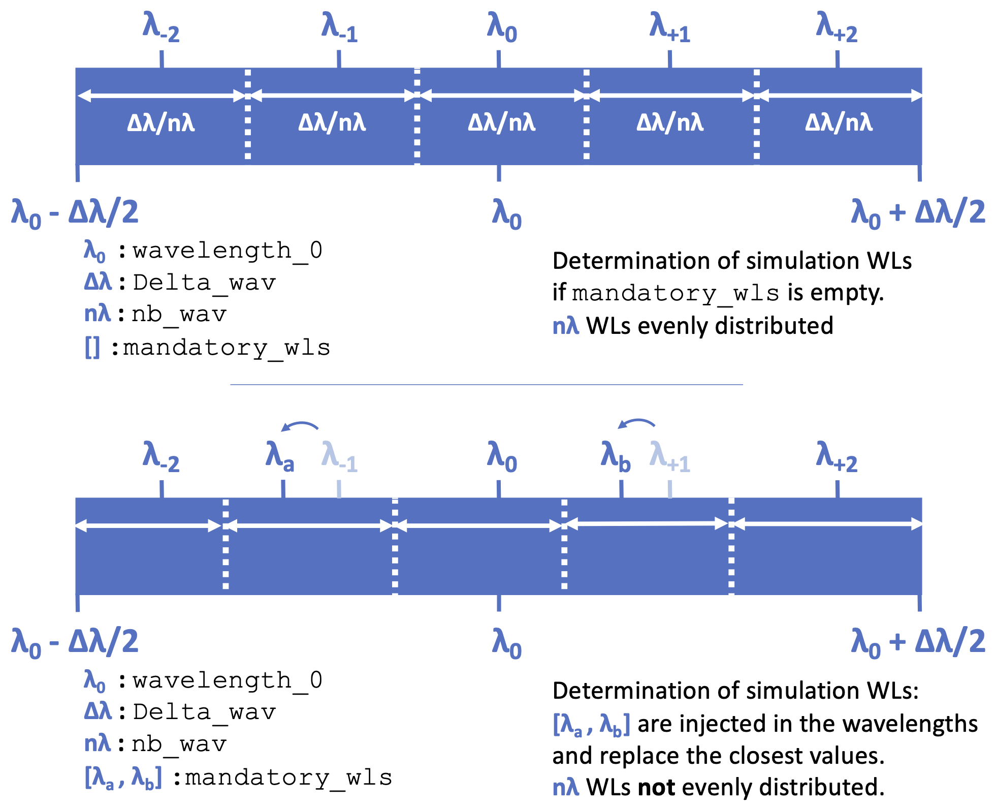
_images/wl_simu.png — Determination of simulation wavelengths `OpticalSystem.wav_vec`

If mandatory_wls is not an empty list, for each mandatory wavelength, we find the closest wavelength in the list and replace it by a mandatory wavelength.

If Delta_wav > 0 and nb_wav > 1, Asterix is automatically in polychromatic wavelength and the following code

PSF = generic_os.todetector_intensity(entrance_EF = input_wavefront)

will return a polychromatic PSF. By default, it is done in all possible simulated wavelengths (wavelengths = OpticalSystem.wav_vec), using the Riemann sum to approximate the polychromatic image. There is also a wavelengths parameter to select other wavelengths. These wavelengths must be sub parts of the simulated wavelengths OpticalSystem.wav_vec because a lot of wavelength specific tools are defined during OpticalSystem initialization. Finally, the normalization in contrast is by default for the whole bandwidth. If you want other wavelengths, use in_contrast=False and measure the PSF to normalize.

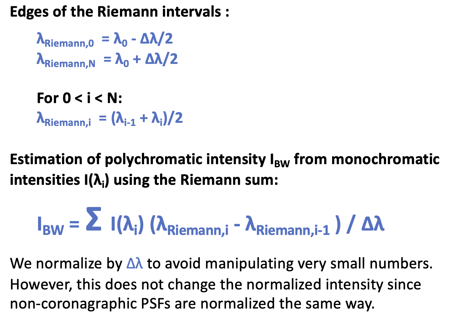
_images/riemann_sum.png — Approximation of a coronagraphic polychromatic Intensity using monochromatic Intensities

Pupil

Pupil is the most simple type of OpticalSystem. It initializes and describes the behavior of single pupil pupil is a sub class of OpticalSystem. Obviously you can define your pupil without that with 2d arrray multiplication (this is a fairly simple object). The main advantage of defining them using OpticalSystem is that you can use default OpticalSystem functions to obtain PSF, transmission, etc… and concatenate them with other elements.

from Asterix.utils import read_parameter_file
from Asterix.optics import  Pupil

config = read_parameter_file(parameter_file)
modelconfig = config["modelconfig"]

pup_round = Pupil(modelconfig)

# Because this is an OpticalSystem, you can access attribute functions:

exit_EF = pup_round.EF_through() # electrical field after the system
                                #(by default, entrance field is 1.)
EF_FP = pup_round.todetector() # electrical field in the next focal plane
PSF = pup_round.todetector_intensity() #  Intensity in the next focal plane

You can define a different radius than the pupil one in the parameter file

pup_round = Pupil(modelconfig, prad = 43)

Some specific aperture types are defined that you can access using the keyword PupType

pup_roman = Pupil(modelconfig, PupType = "RomanPup")

Currently supported PupType are : “RoundPup”, “Clear” (empty pupil plane), “RomanPup”, “RomanLyot”, “RomanPupTHD2”, “RomanLyotTHD2” (same as RomanPup and RomanLyot but with same rotation as on the testbed), “VLTPup”, “SphereApod”, “SphereLyot”.

You can finally defined your own pupils from a .fits using the same keyword if you put a full path. In this case, it will be assumed that the fits file has the same physical size as the entrance pupil defined in the parameter file (diam_pup_in_m). The keyword diam_lyot_in_m is only used in the case of a round Lyot Stop (“RoundPup”) and is not use to scale the .fits files aperture. The pupil in the .fits file are automatically rescaled at 2*prad using binning. Therefore the code requires that the parameter diam_pup_in_pix is a divisor of the .fits file dimension.

Additional details can be found directly in the code documentation.

Coronagraph

Coronagraph is a sub class of OpticalSystem which initializes and describes the behavior of a coronagraph system (from apodization plane at the entrance of the coronagraph to the Lyot plane).

from Asterix.utils import read_parameter_file
from Asterix.optics import Coronagraph

config = read_parameter_file(parameter_file)
modelconfig = config["modelconfig"]
Coronaconfig = config["Coronaconfig"]

corono = Coronagraph(modelconfig, Coronaconfig)

exit_EF = corono.EF_through() # electrical field after the system
                                #(by default, entrance field is 1.)
EF_FP = corono.todetector() # electrical field in the next focal plane
PSF = corono.todetector_intensity() #  Intensity in the next focal plane

Type of coronagraph can be changed with corona_type parameter. Currently supported corona_type are ‘fqpm’ or ‘knife’, ‘classiclyot’ or ‘HLC’. Focal plane functions are automatically normalized in contrast by default. For details about the way to normalize in polychromatic light, see measure_normalization and todetector_intensity documentation in the docs.

Additional details can be found directly in the code documentation.

Deformable Mirror

DeformableMirror is a subclass of OpticalSystem which initializes and describes the behavior of a deformable mirror (DM) system.

from Asterix.utils import read_parameter_file
from Asterix.optics import DeformableMirror

config = read_parameter_file(parameter_file)
modelconfig = config["modelconfig"]
DMconfig = config["DMconfig"]

DM1 = DeformableMirror(modelconfig,
                       DMconfig,
                       Name_DM='DM1',
                       Model_local_dir=Model_local_dir)

You need to provide the influence function .fits file and the distance compared to the pupil plane DM1_z_position In the case of a generic DM (DM1_Generic = True), we need only two more parameter to define the DM: the DM pitch DM_pitch in meters and the number of actuator N_act1D in one of its principal direction. We need N_act1D > diam_pup_in_m / DM_pitch, so that the DM is larger than the pupil. For now we assume that DM_pitch is the same in both direction. The DM will then be automatically defined as squared with N_act1D x N_act1D actuators and the puil centered on this DM. We can also create a specific DM for a given testbed with a file with the relative position of actuators in the pupil and the position of one of them compared to the pupil. This file must have vertical and horizonthal pitch (“PitchV”,”PitchH”) in the header to define the pitch.

Out of the pupil plane DMs are simulated by taking a Angular-Spectrum transform, multiply by the DM phase, and then coming back to a pupil plane. Because we are only in close range, this is more accurate than Fresnel propogation.

Additional details can be found directly in the code documentation.

Concatenate your Optical Systems

This is a particular subclass of Optical System, because we do not know what is inside It can only be initialized by giving a list of Optical Systems and it will create a “testbed” with contains all the Optical Systems and associated EF_through functions.

import from Asterix.utils import read_parameter_file
from Asterix.optics import Pupil, Coronagraph, DeformableMirror, Testbed

config = read_parameter_file(parameter_file)
modelconfig = config["modelconfig"]
Coronaconfig = config["Coronaconfig"]
DMconfig = config["DMconfig"]

pup_round = Pupil(modelconfig)

DM34act = DeformableMirror(modelconfig,
                           DMconfig,
                           Name_DM='DM1',
                           Model_local_dir=Model_local_dir)

DM32act = DeformableMirror(modelconfig,
                           DMconfig,
                           Name_DM='DM3',
                           Model_local_dir=Model_local_dir)

corono = Coronagraph(modelconfig, Coronaconfig)
# and then just concatenate
testbed = Testbed([pup_round, DM34act, DM32act, corono],
                  ["entrancepupil", "DM1", "DM3", "corono"])

The whole point of this system is that it can be easily changed. For example, we can add another DM32act DM just like that:

testbed = Testbed([pup_round, DM34act, DM32act, DM32act, corono],
                  ["entrancepupil", "DM1", "DM3", "DM4", "corono"])

or a specific pupil in the entrance plane of the coronagraph (e.g. like the Roman configuration).

pup_roman = Pupil(modelconfig, PupType = "RomanPup")
testbed = Testbed([pup_round, DM34act, DM32act,pup_roman, corono],
                  ["entrancepupil", "DM1", "DM3", "romanpupil" , "corono"])

Additional details can be found directly in the code documentation.